3 Effect Sizes

3.1 Introduction

This chapter explains the importance of effect sizes in research, and summarises some of the main ways in which effect sizes can be calculated and reported.

Effect sizes are statistical measures that quantify the magnitude and practical significance of relationships, or differences, between variables in research studies.

Unlike statistical significance (p-values), which can be influenced by sample size, effect sizes provide a standardised way to evaluate the practical importance of research findings.

Effect sizes are very useful because they:

Help us understand the practical significance of our findings;
Allow for meaningful comparisons across different studies;
Provide essential information for meta-analyses and systematic reviews;
Complement traditional statistical testing by focusing on magnitude, rather than just statistical significance.

3.2 Effect Sizes - Definition and Purpose

3.2.1 Introduction

Effect sizes help us measure the difference in the means of our experimental and control groups.

Effect sizes quantify the strength or magnitude of a relationship or difference in a data analysis, independent of sample size.

They provide a standardised metric to assess practical significance, complementing statistical significance. This ensures we understand the real-world impact of our findings.

3.2.2 Why do effect sizes matter?

It’s often argued that effect sizes matter more than statistical significance because:

Statistical significance (p-values) can be achieved with large enough samples, even when effects are trivially small;
Effect sizes tell us about practical importance - whether a finding matters in the real world;
They allow direct comparison between analyses or studies using different measures or scales;
Effect sizes help inform policy decisions by showing the actual magnitude of impact.

Consider this example: A study might find a “statistically significant” difference between two teaching methods (p < .05), but if the effect size is tiny (d = 0.01), the real-world benefit of changing methods would be negligible. This illustrates why focusing solely on significance can be misleading.

3.2.3 Practical significance of effect sizes

‘Practical significance’ refers to the real-world importance or meaningfulness of a research finding, effect, or outcome.

Unlike statistical significance, which focuses on whether results are likely due to chance, practical significance evaluates whether the results matter in a meaningful way for decision-making, policy, or real-world applications.

This concept is particularly important because:

not all statistically significant findings have meaningful real-world implications;
decision-makers need to understand the actual impact of interventions or changes; and
arguably, resources and efforts should be directed toward changes that make a meaningful difference.

When assessing practical significance, we consider factors such as:

the magnitude (size) of the effect or change;
the context and setting where the results will be applied;
the costs and benefits associated with implementation; and
the relevance to stakeholders and end-users.

3.2.4 Standardisation

Standardisation refers to the process of transforming measurements or scores into a common scale that allows for meaningful comparisons.

When discussing effect sizes, standardisation typically involves expressing differences or relationships in terms of standard deviation units, making results comparable across different measures, scales, or studies.

This transformation is essential because raw scores or differences may be difficult to interpret when variables are measured using different scales or units. For instance, comparing the impact of an intervention on test scores measured from 0-100 with another measured from 1-5 would be challenging without standardisation.

Why does standardisation matter?

Standardisation plays a crucial role in understanding and interpreting effect sizes, particularly when comparing results across different studies or contexts.

Effect sizes, such as Cohen’s d, provide this standardised measure of the magnitude of an observed effect, independent of sample size. This allows us to quantify the strength of relationships or differences in a way that is not merely reliant on statistical significance, which can be influenced by sample size.

For example, Cohen’s d calculates the difference between two means relative to the standard deviation of the data, providing a scale-free measure that can be universally interpreted, thus facilitating meta-analyses and broader comparisons across diverse research findings.

The use of standardised effect sizes enhances the reproducibility and comparability of scientific research. By expressing the size of an effect in standardised units, we can more easily determine how substantial the effect is in practical terms (e.g., clinical significance or practical implications).

This is particularly important in fields (like psychology and education) where interventions might show statistically significant results but differ widely in their real-world impact.

Standardised effect sizes thus serve as a “common language”, helping to bridge the gap between statistical results and practical outcomes, and ensuring that decisions based on research findings are informed by a clear understanding of the effect’s magnitude.

3.2.5 Magnitude of effect

In the context of effect sizes, the term “magnitude of effect” refers to the quantitative measure of the strength or size of a relationship or difference between variables within a study.

This helps to determine how significant and impactful a finding is from a practical standpoint, beyond just statistical significance (which merely tells us whether an effect exists or not).

Remember: effect sizes provide a standardised way to express the difference between groups or the association between variables, making it easier to compare results across different studies or different conditions within the same study.

The magnitude of the effect can be categorised as “small”, “medium”, or “large”, based on established benchmarks. This categorisation helps us understand and report the practical significance of our results:

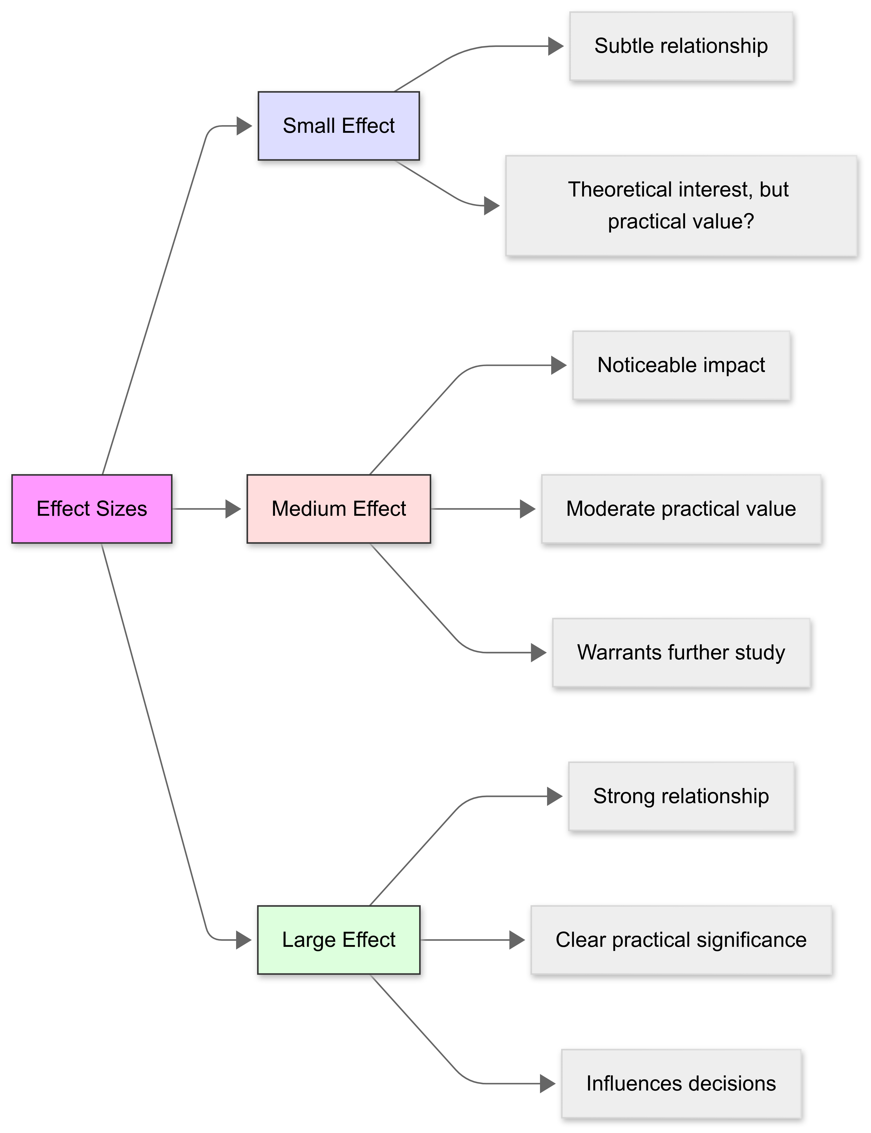
Descriptions of effect sizes, based on Cohen (1988).

The magnitude of effect is essential for understanding the relevance and utility of research findings, especially when deciding if the outcomes of interventions or studies have meaningful implications in real-world scenarios.

For example, in clinical research, a “large” effect size on a treatment’s efficacy might lead to changes in medical practice, whereas a “small” effect size might be considered insufficient to justify a change in treatment protocols.

3.2.6 A complement to p-values

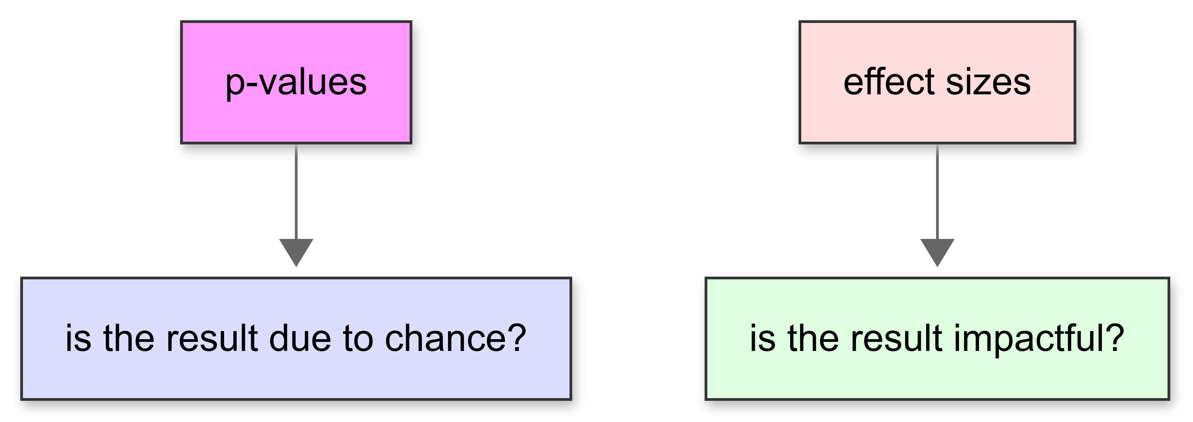
Effect sizes and p-values are both used to analyse data, and they work together to provide a fuller understanding of study results.

While p-values tell you whether the results of your study are likely to be due to chance, effect sizes give you an idea of how large or important those results are.

p-values

A p-value helps you determine whether an observed effect is statistically significant:

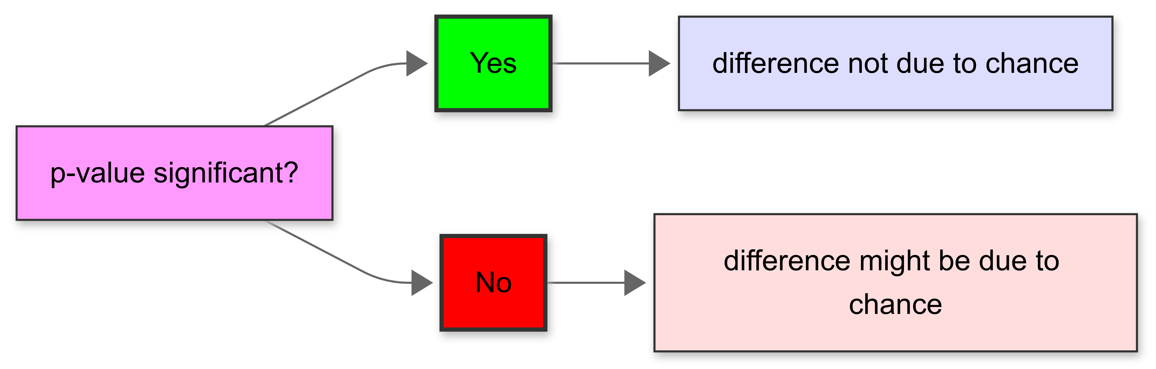
For instance, in a medical trial, if a p-value is very small (<0.05, for example), it suggests that the difference in recovery rates between a treatment group and a control group is not just due to random chance.

However, the p-value doesn’t tell you anything about the size of the difference between the groups; whether it’s big enough to be important in a real-world setting.

Effect sizes

This is where effect sizes come in. They measure the strength of the relationship between variables or the magnitude of differences between groups. So, even if a p-value shows that there is a statistically significant difference, an effect size can tell you whether that difference is small, medium, or large.

This is crucial because a statistically significant result could still have a very small effect size, meaning it might not be practically important.

For example, a medication might be proven to statistically significantly improve recovery times compared to a placebo, but if the effect size is small, the actual amount of time saved might be minimal, say one day faster than usual. Knowing this, doctors and patients might decide that the side effects of the medication aren’t worth the gain.

So, while p-values can tell you if an effect exists, effect sizes tell you how much it matters. They complement each other by providing a complete picture of both the reliability and relevance of research findings.

3.3 Measuring Effect Sizes

3.3.1 Introduction

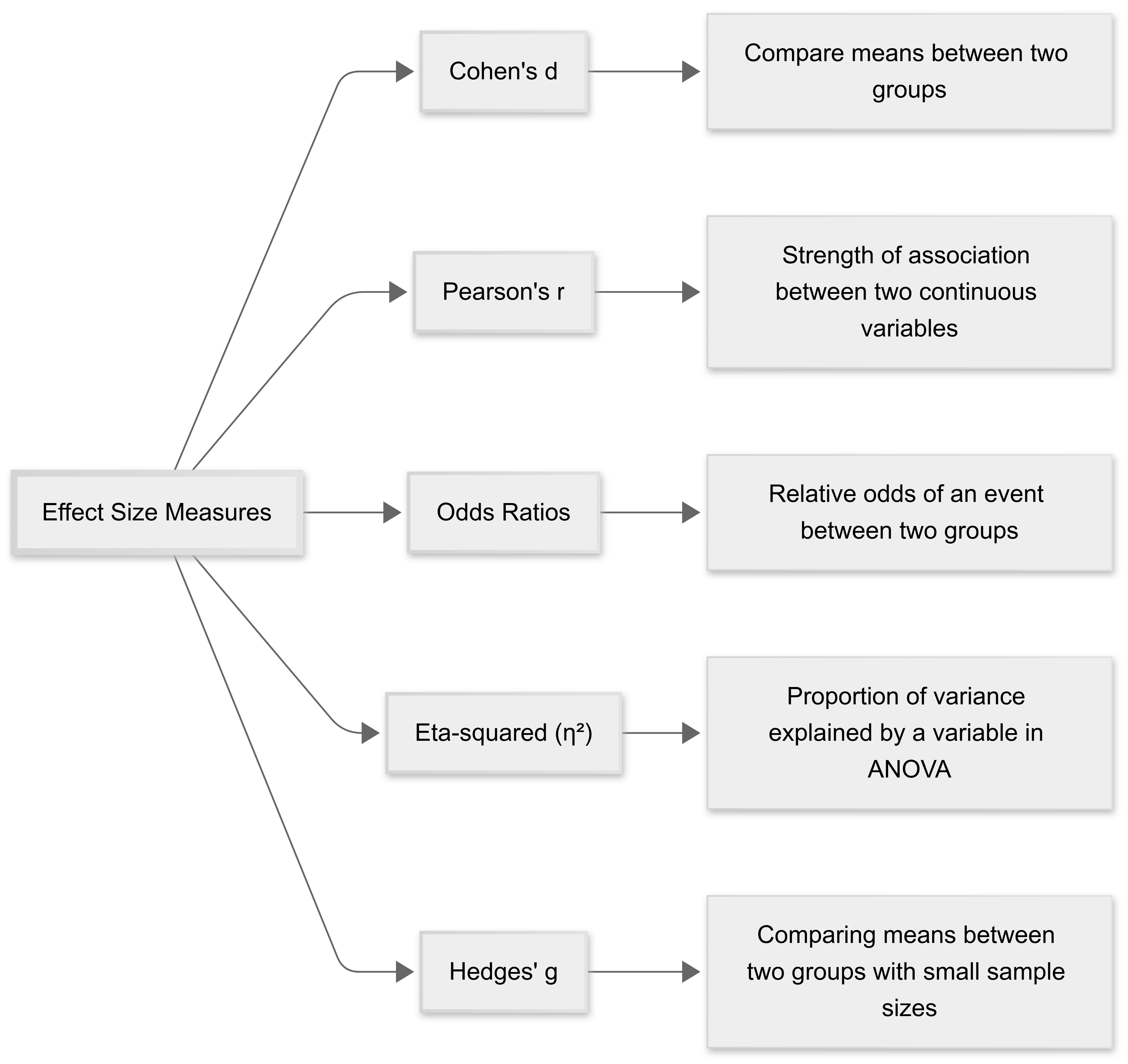
There are a few different ways we can measure effect size. Different measures are suited to different contexts.

Common measures include Cohen’s d for mean differences, Pearson’s r for correlations, odds ratios for categorical outcomes, and eta squared for variance explained in ANOVA.

Selecting the appropriate effect size depends on the data and research question.

3.3.2 Cohen’s d

Introduction

Cohen’s d (Cohen, 1988) is a popular effect size measure used to express the standardised difference between two means.

It’s calculated by subtracting the mean of one group from the mean of another and dividing the result by the pooled standard deviation of the groups.

Formula

\[ d = \frac{M_1 - M_2}{s_p} \] Where:

$M₁$ and $M₂$ are the means of the two groups
$s_p$ is the pooled standard deviation

Advantages

Cohen’s d is independent of sample size (unlike statistical significance);
It allows comparison across different studies or analyses;
It’s useful for meta-analyses (see below); and
It helps us determine practical significance of findings

Limitations

However, Cohen’s d assumes our data is normally distributed;
It’s sensitive to outliers; and
Context-dependent interpretation is necessary - a ‘small’ effect could still be important!

When is it useful?

Cohen’s d is particularly useful in gauging the extent of an effect where the variable of interest is continuous and normally distributed.

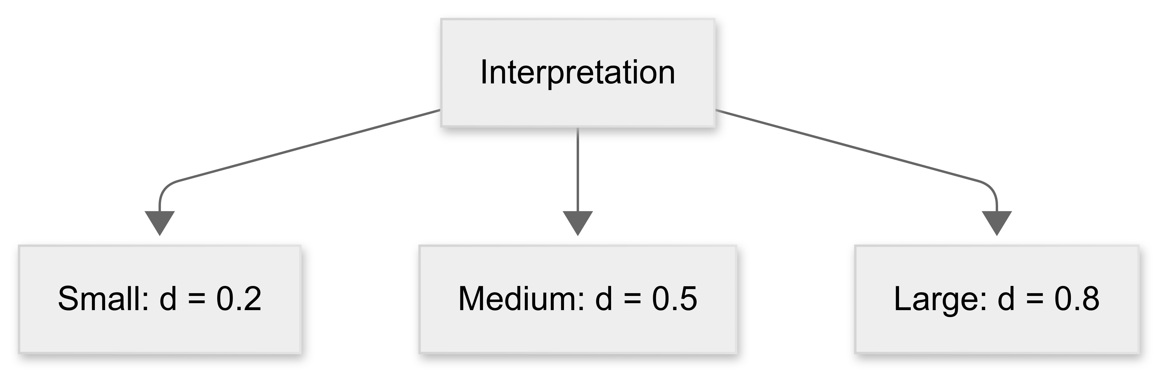
Cohen’s d values of 0.2, 0.5, and 0.8 are typically interpreted as “small”, “medium”, and “large” effects, respectively, providing an easy-to-understand benchmark for evaluating the practical significance of findings.

3.3.3 Pearson’s r

Scatterplots of positive, negative, and no correlation.

We’ve already encountered Pearson’s r in the context of correlation analysis. Note that, like Cohen’s d, it’s also a measure of effect size.

In this case, Pearson’s r is used to explore effect sizes when the research focus is on understanding the strength and direction of a linear relationship between two continuous variables.

Remember: Cohen’s d is used to measure the size of the difference between two means. Correlation is about association.

This correlation coefficient is particularly useful in situations where it’s important to measure how much one variable predicts or is associated with another.

3.4 Interpreting Pearson’s r effect sizes

Cohen (1988) proposed the following guidelines for interpreting the magnitude of correlations:

	Correlation coefficient (r)		Effect Size
	± .10		Small effect
	± .30		Medium effect
	± .50		Large effect

Note that these are rough guidelines and should be interpreted within the context of your research field. Some disciplines may have different conventions for what constitutes a meaningful effect size.

The sign (+ or -) indicates the direction of the relationship:

Positive correlations (+): As one variable increases, the other tends to increase
Negative correlations (-): As one variable increases, the other tends to decrease

The value can range from -1 (perfect negative correlation) to +1 (perfect positive correlation), with 0 indicating no linear relationship.

3.4.1 Odds ratio

Introduction

The odds ratio is a measure of effect size that describes the ratio of the odds of an event occurring in one group to the odds of it occurring in another group.

Commonly used in case-control studies, and particularly in medical and epidemiological research, the odds ratio helps quantify how strongly the presence or absence of a property affects the outcome of interest.

An odds ratio greater than 1 indicates increased odds of the event occurring with the property, less than 1 indicates decreased odds, and an odds ratio of 1 indicates no effect.

Example - selecting a coloured ball

Imagine you have two boxes of with a mixture of red and blue-coloured balls. You want to see which box has more red balls compared to blue balls.

The first box has a lot of red balls and just a few blue ones. The second box has some red balls, but it has more blue balls than the first box. To understand how much more likely it is to pick a red ball from the first box than from the second box, we can use the odds ratio.

If the odds ratio number is bigger than 1, it means you’re more likely to pick a red ball from the first box compared to the second one.
If the number is exactly 1, it means both boxes have the same chance of picking a red ball.
And if the number is less than 1, you are less likely to pick a red ball from the first box than from the second one.

So, the odds ratio helps us see which box makes it easier to pick a red ball.

Example - injury prevention in football players

Imaging a sports scientist wants to evaluate the effectiveness of a new injury prevention training program. They implement a study involving two groups of football players:

Group A: Players who participated in the program (the treatment group).
Group B: Players who did not participate in the program (the control group).

When they analyse their data, they see that:

Group A (Treatment group): 10 out of 100 players sustained injuries.
Group B (Control group): 30 out of 100 players sustained injuries.

They calculate the odds for each group:

Odds of injury in Group A:

\[ \text{Odds} = \frac{\text{Number Injured}}{\text{Number Not Injured}} = \frac{10}{90} = 0.111 \]

Odds of injury in Group B:

\[ \text{Odds} = \frac{\text{Injured}}{\text{Not Injured}} = \frac{30}{70} = 0.429 \]

Then, they calculate the odds ratio:

\[ \text{Odds Ratio} = \frac{\text{Odds in Group A}}{\text{Odds in Group B}} = \frac{0.111}{0.429} \approx 0.26 \]

On the basis of the odds ratio, the sports scientist concludes:

An OR of 0.26 means the odds of injury for players in the program (Group A) are 74% lower than for players who did not participate (Group B).
This suggests the injury prevention program appears to be effective, as the effect size of the treatment can be said to be 74%.

Reporting Odds Ratios

When reporting odds ratios in research, it’s important to include several key elements:

The odds ratio value should be reported with confidence intervals (typically 95% CI)
Include the p-value to indicate statistical significance
Provide a clear interpretation of the effect size magnitude:
- OR = 1.68 to 3.47: Small effect
- OR = 3.47 to 6.71: Medium effect
- OR > 6.71: Large effect

Example reporting format:

“The odds ratio for injury prevention was OR = 0.26, 95% CI [0.18, 0.37], p < .001, indicating a large protective effect of the training program.”

Note that for odds ratios less than 1 (indicating decreased odds), you can convert them to their reciprocal (1/OR) when discussing effect size magnitude. In our example, 1/0.26 = 3.85, which would indicate a medium-sized effect.

3.4.2 Eta squared

Introduction

Eta squared ($η²$) is an effect size measure used in the context of variance analysis.

$η$² (pronounced “AY-tuh”)represents the proportion of the total variance in a dependent variable that is attributable to a factor or an independent variable. Eta squared values range from 0 to 1, where higher values suggest a greater effect of the independent variable on the dependent variable.

$η²$ is commonly used in ANOVA tests, providing insights into the importance of different factors in experimental designs and helping researchers understand the extent of an effect.

Formula

\[ η² = \frac{SS_{effect}}{SS_{total}} \]

where SS_effect is the sums of squares for the effect of interest and SS_total is the total sums of squares.

Interpretating η²

Like Cohen’s d, effect sizes for η² can be categorised as “small” (≈0.01, explaining 1% of the variance), “medium” (≈0.06, explaining 6% of the variance), and “large” (≈0.14, explaining 14% of the variance).

$η²$ is useful as it is easy to calculate and interpret, it provides a standardised measure of effect size, and is useful for comparing effects across studies.

However, $η²$ can be positively biased, especially with small samples. It may overestimate population effects, and partial η² ($η²p$) is often preferred for designs with multiple factors.

Note: When reporting eta squared in research, it’s important to include both the η² value and its interpretation in terms of effect size magnitude. This helps readers understand the practical significance of your findings.

Example

A sports analyst wants to investigate the effect of three different swimming training programs on swim speed (measured in seconds to complete a 100-meter freestyle).

Their goal is feed back to the coach how much of the variation in swim speed is explained by the training program.

They conduct an empirical study:

The Independent Variable (IV) is the training program (3 levels: Sprint-focused, Endurance-focused, Mixed training).
The Dependent Variable (DV) is the recorded swim speed (time to complete 100m freestyle in seconds).
They recruit some participants (45 swimmers) and allocate 15 per training program.

The swimmers are tested before and after an 8-week training period, and their improvement in swim speed is recorded. An ANOVA is conducted to compare the mean improvements in swim speed across the three training groups.

The ANOVA produces the following:

Between-group variance: This is the variance explained by the training programs.
Total variance: This is the total variance in swim speed improvement across all swimmers.

Now, the analyst calculates eta-squared:

\[ \eta^2 = \frac{\text{Sum of Squares Between Groups}}{\text{Total Sum of Squares}} \]

Imagine the results are:

Sum of Squares Between Groups = 120
Total Sum of Squares = 200

Then:

\[eta^2 = \frac{120}{200} = 0.60\]

How will the analyst interpret this and report back to the coach?

An $η²$ value of 0.60 means that 60% of the variance in swim speed improvement can be attributed to the type of training program.
This indicates that the training program has a substantial effect on swim speed improvements

3.4.3 Hedge’s g

Hedge’s g is a measure of effect size used to quantify the difference between two means, similar to Cohen’s d, but with an adjustment for small sample sizes.

It standardises the mean difference by dividing it by the pooled standard deviation and includes a correction factor to reduce bias when sample sizes are small.

This makes Hedge’s g particularly useful in studies with limited data or when conducting meta-analyses to ensure accurate comparisons across studies.

Example

Scenario:

A sports scientist wants to investigate the effect of a new agility training program on badminton players’ reaction times. Their aim is to compare the reaction times of players who underwent the agility training program with those who followed their standard training routine.

Study Design:

Independent Variable: Type of training (Agility Training Program vs. Standard Training Routine).
Dependent Variable: Reaction time (measured in milliseconds).
Participants: 30 players (15 in each training group).

Data Collection:

After an 8-week training period, players’ reaction times are measured. Due to the small sample size, Hedges’ g is used to calculate the standardised mean difference between the two groups, adjusting for sample size bias.

Formula for Hedges’ g

\[g = \frac{\overline{X}_1 - \overline{X}_2}{s_p}\]

Where:

$\overline{X}_1$ is the mean of group 1
$\overline{X}_2$ is the mean of group 2
$s_p$ is the pooled standard deviation, calculated as:

\[ s_p = \sqrt{\frac{(n_1 - 1)s_1^2 + (n_2 - 1)s_2^2}{n_1 + n_2 - 2}} \]

Example calculation

Suppose the results are:

Mean reaction time for the agility training group $overline{X}_1$: 250 ms
Mean reaction time for the standard training group $overline{X}_2$: 275 ms
Standard deviations: s_1 = 15ms, s_2 = 20ms
Sample sizes: n_1 = 15, n_2 = 15

First, we calculate the pooled standard deviation:

\[ s_p = \sqrt{\frac{(15 - 1)(15^2) + (15 - 1)(20^2)}{15 + 15 - 2}} = \sqrt{\frac{14 \cdot 225 + 14 \cdot 400}{28}} = \sqrt{\frac{3150 + 5600}{28}} = \sqrt{312.5} \approx 17.68 \]

Now we can calculate Hedges’ g:

\[ g = \frac{250 - 275}{17.68} = \frac{-25}{17.68} \approx -1.41 \]

Interpretation

A Hedges’ g of -1.41 indicates a large negative effect size, meaning the agility training program substantially reduced reaction times compared to the standard training routine.

Note: the negative sign reflects that the mean reaction time for the agility training group was smaller (better) than that of the standard training group.

3.5 Interpreting Effect Sizes

3.5.1 Introduction

Interpreting effect sizes involves comparing their values to established benchmarks, or considering the context of the study.

As we’ve noted:

Cohen’s d categorises effects as ‘small’, ‘medium’, or ‘large’;
Correlation coefficients are interpreted based on their strength and direction.

Earlier, we noted that this is one of the advantages of using effect sizes: they give us a fairly straightforward way of communicating whether our results, even if significant, are important or not.

3.5.2 Benchmarks for interpretation

As we’ve noted, effect sizes are standardised metrics that facilitate the interpretation of research findings across various contexts and studies.

Benchmarks for interpreting these sizes, such as Cohen’s conventions (small = 0.2, medium = 0.5, large = 0.8), provide a general guideline.

However, the relevance of these benchmarks can vary significantly depending on the field of study and the specific context.

For example, in fields like clinical psychology, a small effect size can still be of great practical significance if the treatment under consideration is the only one available, or has minimal side effects compared to alternatives that might have a bigger effect size.

3.5.3 Small, medium, large thresholds

The classification of effect sizes into small, medium, and large is important for assessing the magnitude of an effect.

These thresholds are immensely helpful to researchers, practitioners, and policymakers as they attempt to understand the potential impact of their findings in a clear and standardised way.

It’s important to note that these categories are not absolute and should be viewed as part of a broader interpretative framework that considers the specific conditions and variables of each study.

For instance, in educational research, a small effect size on a new teaching method could still translate to significant improvements when applied across large populations.

3.5.4 Direction of effect

The direction of an effect size is as important as its magnitude. This refers to whether the effect is positive or negative, indicating the direction of the relationship between variables or the difference between groups.

Understanding the direction helps in making precise conclusions about the nature of the effect and its potential implications.

For example, a negative effect size in a drug efficacy study would indicate that the treatment is less effective than the control, which is critical for clinical decision-making and policy guidelines.

3.5.5 Clinical and practical implications

Interpreting effect sizes in terms of their practical implications is vital as we attempt to translate research findings into real-world applications. Especially when dealing with people!

Even a small effect size can have significant implications if the outcome measure is crucial for public health or policy.

Those making decisions must consider both the magnitude and the direction of effect sizes to make informed decisions that can lead to effective interventions and improved outcomes.

3.6 Reporting Effect Sizes

Throughout this section, we’ve emphasised that effect sizes should be calculated alongside our hypothesis tests, and reported along with significance to ensure transparency and replicability.

Proper reporting includes the formula used, raw data, and confidence intervals for the effect size.

3.6.1 Reporting guidelines

When reporting effect sizes, include the following elements:

A clear definition of the effect size measure used.
The calculated effect size value.
Contextual explanation of what the effect size value indicates about the relationship or difference studied.

You should adhere to the reporting standards set by the American Psychological Association (APA) or other relevant bodies, ensuring that all necessary details are included for clarity and transparency.

Here’s an example (based on APA format):

A one-way ANOVA was conducted to examine the effect of study method (group study, individual study, no study) on test performance. The results showed a significant effect of study method on test scores, F(2, 57) = 8.45, p = .001, η² = .23, indicating that 23% of the variance in test scores was explained by the study method. Post hoc Tukey tests revealed that group study (M = 85.4, SD = 5.2) resulted in significantly higher scores than no study (M = 72.1, SD = 6.4), p < .001, while individual study (M = 79.8, SD = 5.8) did not significantly differ from either group study or no study.

3.6.2 Confidence intervals

Confidence intervals (CIs) for effect sizes add value by providing a range within which the true effect size is likely to fall.

Note: they’re not always required (this will depend on discipline and journal/conference).

However reporting CIs helps in assessing the precision of the estimated effect sizes and the statistical significance of the results.

For example, an effect size with a 95% CI that doesn’t include zero is typically considered statistically significant.

3.6.3 Replicability

As you know, replicability (repeating studies) is critical in scientific research. Detailed reporting of effect size calculations (including software or tools used), the specific formulas, and any assumptions made during the calculations, supports the replicability of the findings and helps researchers/analysts who are replicating your work to evaluate its ‘replicability’.

You are always are encouraged to provide complete information, enabling others to perform similar analyses to yours, and verify your results.

3.7 Effect Sizes in Meta-Analysis

3.7.1 Introduction

Effect sizes are integral to meta-analyses, where they enable us to combine and compare results across studies.

A meta-analysis is a systematic statistical procedure that combines data from multiple independent studies to estimate the overall effect of a particular intervention or relationship.

It represents a higher level of analysis that goes beyond individual research findings to identify patterns, consistencies, and variations across studies.

This approach helps researchers draw more robust conclusions by increasing statistical power and providing more precise effect estimates than could be achieved through single studies alone.

3.7.2 Aggregating research studies

Introduction

‘Meta-analysis’ is a powerful research tool that combines results from multiple independent studies to draw broader conclusions and identify patterns across research.

By systematically aggregating findings from various studies, researchers can:

Increase statistical power and precision of effect estimates;
Resolve conflicts between contradictory studies;
Identify trends and patterns across different contexts; and
Generate more generalisable conclusions.

What do meta-analyses involve?

The process typically involves:

Systematic literature review to identify relevant studies
Assessment of study quality and eligibility
Extraction of effect sizes and statistical data
Statistical synthesis of results
Analysis of heterogeneity and potential moderators

There are specific software tools designed to assist with conducting meta-analyses (e.g., RevMan, and the Metafor/Meta packages within R).

Meta-analyses are particularly valuable in evidence-based practice, as they sit at the top of the evidence hierarchy, providing comprehensive summaries of available research on specific topics.

Key Challenge: Not all studies can be directly compared. We must carefully consider methodological differences, study quality, and potential sources of bias when aggregating research.

3.7.3 Standardised metrics

As we’ve noted, one of the major strengths of using effect sizes is that they provide a standardised metric by which we can compare different studies.

These metrics convert study results into a common scale, making it possible to:

Compare outcomes across diverse studies
Pool results meaningfully in statistical analyses
Interpret the magnitude of effects consistently

In terms of effect sizes, common standardised metrics include:

Standardised Mean Difference (Cohen’s d, Hedges’ g)
Correlation Coefficients (r, Fisher’s z)
Odds Ratios and Risk Ratios

As in single studies, our choice of standardised metric in meta-analyses depends on:

The type of data available from primary studies
The research question being addressed
The intended audience and ease of interpretation

3.7.4 Combining results

Introduction

Combining effect sizes in meta-analyses involves integrating the findings from multiple studies into a single, comprehensive statistical summary. This process results in an overall conclusion about the effect under investigation, based on varied research outcomes.

Step One

The first step in combining effect sizes is to calculate the standardised effect size for each individual study. This involves transforming the study’s results into a common metric, such as Cohen’s d, Pearson’s r, or odds ratios, depending on the nature of the data and the study design. This standardisation allows different studies to be comparable despite variations in scale or measurement methods.

Step Two

Once each study’s effect size is standardised, the next step is to aggregate these values. This is typically done using a weighted average, where the weight given to each study’s effect size is inversely proportional to the variance of the effect size estimate. This weighting ensures that studies with larger sample sizes, which generally provide more precise estimates, have a greater influence on the overall effect size than smaller studies.

The choice of model for combining effect sizes, either a fixed-effect or a random-effects model, depends on the extent of heterogeneity among the studies’ effect sizes. A fixed-effect model assumes that all studies are sampling from the same true effect, while a random-effects model allows that the true effect might vary between studies.

Step Three

Finally, researchers must assess the heterogeneity of the effect sizes using statistical tests (such as Cochran’s Q test and by calculating the [I^2 statistic]. This step is crucial for determining whether the studies are sufficiently similar to warrant combining their results and for interpreting the validity of the aggregated effect sizes.

If significant heterogeneity is present, it may be necessary to explore potential moderators or conduct subgroup analyses to understand the sources of variation among the study results.

3.7.5 Assessing heterogeneity

Introduction

In the context of meta-analyses, assessing heterogeneity in effect sizes is crucial for understanding the variability among the results of different studies that are pooled together.

This helps determine whether the effect sizes from the individual studies differ more than would be expected by chance alone and provides insights into the consistency and generalizability of the findings across various settings, populations, or conditions.

Assessing Heterogeneity in Effect Sizes

Statistical Tests for Heterogeneity:

Q Test (Cochran’s Q): This test provides a statistic that measures the total deviation of individual study effects from the overall effect estimated by the meta-analysis. A significant Q value suggests the presence of heterogeneity among the effect sizes.
I² Statistic: The I² statistic quantifies the proportion of total variation across studies that is due to heterogeneity rather than chance. Values of I² can be interpreted as follows: 0% indicates no observed heterogeneity, 25% low, 50% moderate, and 75% high heterogeneity.

Visual Inspection:

Forest Plots are commonly used to display the effect sizes from individual studies in a meta-analysis and include a measure of variability (usually confidence intervals). If the confidence intervals of different studies overlap significantly, it suggests less heterogeneity. Wide variance in the placement of effects on the plot indicates more heterogeneity.

Example of a visualisation for a meta-analysis.

Why Assess Heterogeneity in effect sizes?

Understanding heterogeneity helps researchers determine whether the findings from a meta-analysis can be generalized across various study populations or settings. High heterogeneity might suggest that the effect size varies substantially under different conditions, which could limit the generalisability.

Analysing heterogeneity can also lead to the detection of subgroup effects, where certain groups may respond differently. This is important in tailoring interventions or treatments based on specific characteristics of subgroups.
Significant heterogeneity prompts researchers to explore what factors might contribute to the variability. This can guide further studies to explore aspects such as demographic differences, variations in intervention implementation, or other methodological differences between the studies.
Assessing and understanding heterogeneity can help in refining theoretical models about the relationships being studied. It may indicate that existing models need modification to accommodate diverse conditions or populations.

In summary, heterogeneity assessment in meta-analyses is vital for ensuring the accuracy, relevance, and applicability of the synthesised conclusions. It helps in recognizing the limits of the findings and in identifying areas where more research is needed or where tailored approaches might be required.

3.7.6 Generalisation of findings

Finally, in meta-analyses, effect sizes are essential for combining and comparing the findings from multiple studies. This standardisation allows us to synthesise varying outcome measures into a common metric, regardless of the original measures used.

By doing so, effect sizes facilitate a clearer understanding of the overall impact or association across different contexts, making the aggregated results more comprehensive and reliable. They also adjust for differences in sample sizes across studies, giving more weight to larger studies which tend to be more precise. This weighting is critical as it helps ensure that the overall results are not unduly influenced by smaller, potentially less accurate studies.

Effect sizes help in evaluating the consistency of results across various studies, which is crucial for generalising findings. By assessing the average effect size and its variability (heterogeneity), researchers can gauge how stable an effect is across different settings or populations. This aids in understanding whether the observed effects are robust and applicable in different or broader contexts beyond the specific conditions of individual studies.

So, effect sizes in meta-analyses don’t just enhance the statistical power to detect effects but also strengthen the external validity of conclusions, supporting generalisation to a wider audience or application under varied circumstances.

3.8 References

Cohen, J. (1988). Statistical Power Analysis for the Behavioral Sciences (2nd ed.). New York, NY: Routledge Academic.